Penalty Functions
Created on: 2024-12-08
Tags: #PenaltyFunctions
Course: Optimization
Definition
Penalty Function methods are used to solve constrained NLP which reduces the problem into a series of unconstrained optimization problems.
They use unconstrained optimization techniques like Cauchy’s method, DFP, BFGS, FR, etc.
There are two types of penalty functions:
- Interior penalty functions
- Exterior penalty functions
Interior penalty functions Here, the Kuhn Tucker necessary conditions are modified to,
$\nabla f(x) + u\,\nabla g(x) = 0$ $g(x) \le 0$ $u \ge 0$ $u\,g(x) = -t$
Using the modified conditions, we can obtain \(\nabla(f - t\log(-g(x))) = 0\) Thus, the constrained problem can be transformed as a unconstrained problem i.e. \(\text{Minimize}\,\,\, f(x) - t\,\log(-g(x))\) This can be solved using the unconstrained optimization techniques. The unconstrained minima lies in the feasible region and converges to the solution as $t$ is varied.
Algorithm
- Select a large value of $t$, which boils down the problem to minimization of $g(x)$. Since, $f(x) < t\log(-g(x))$ for very large value of $t$.
- Solve the problem for that value of $t$.
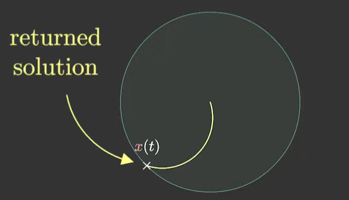
- Obtain the value of $x(t)$.
- Now, take $t_{i+1} = c\,t_{i}$, where $c$ is a number between 0 and 1.
- Go to step 2 and continue till $\Delta f(X_{i})\%<\epsilon$, where $\epsilon$ is a very small positive number.
Exterior Penalty functions
Using the modified conditions, we can obtain \(\nabla(f + t\,(max[\,0,\,g(x)\,])^2) = 0\) Thus, the constrained problem can be transformed as a unconstrained problem i.e. \(\text{Minimize}\,\,\, f(x) + t\,(max[\,0,\,g(x)\,])^2\) This can be solved using the unconstrained optimization techniques. The unconstrained minima lies in the infeasible region and converges to the solution as $t$ is varied.
Algorithm
- Select a small value of $t$.
- Solve the problem for that value of $t$.
- Obtain the value of $x(t)$.
- Now, take $t_{i+1} = c\,t_{i}$, where $c$ is a number greater than 1.
- Go to step 2 and continue till $\Delta f(X_{i})\%<\epsilon$, where $\epsilon$ is a very small positive number.
Linked from
- No other published notes link here yet.