Turbulence Modelling
Created on: 2024-12-30
Tags: #RANS #TurbulenceModelling
Course: SU2
Reynolds Averaged Navier Stokes
Replacing the statistical definition of the flow quantities in the Navier-Stokes Equation (Momentum Equation), we get the RANS equations. \(A(t) = \bar{A} + A'(t)\) Where $A(t)$ is some time-varying quantity and $\bar{A}$ is the time-average of the quantity whereas the $A’(t)$ is the variation of the quantity about the average in time.
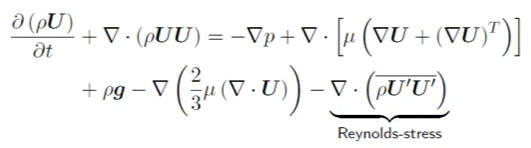
The most common approach for modelling the Reynold’s stress term is the Boussinesq hypothesis. \(-\overline{\rho U'U'} = \mu_{t}(\nabla U + (\nabla U)^T) - \frac{2}{3}\rho kI - \frac{2}{3}(\nabla \cdot U)I\) So, $\mu_{t}$ needs to be calculated to close the equations.
Mixing Length Models
- Older models used a mixing length ($l_{m}$) approach to calculate the eddy viscosity ($\mu_{t}$).
- The wall blocks the maximum size of the eddies.
- Prandtl mixing length hypothesis supposes that \(l_{m} = \kappa y,\,\,\, \kappa=0.41\)
Van Driest Mixing Model
- The viscosity in the viscous sub-layer dampens the eddies and reduces their size.
The scale of turbulence
- The mixing length is specified algebraically, thus is fixed throughout the domain as distance from a geometry is fixed. \(\mu_{t} = \rho k^{0.5} l_{m}\)
- We solve a transport equation for $\epsilon$.
- Instead of $l_{m}$, solve for $\epsilon$ (Turbulence Dissipation Rate): \(\mu_{t} = C_{\mu} \frac{\rho k^2}{\epsilon}\) Hence, we have the k-Epsilon model.
Linked from
- No other published notes link here yet.